LaTeX Graphics

Overview \| The picture Environment \| The pstricks Package
LaTeX Graphics	The picture Environment	LaTeX Graphics

Contents Basics Line segments Circles Arrows The multiput and the linethickness command Ovals, thinlines, thicklines Text, formulas, colors Quadratic Bézier curves Marking angles Line thickness again: the linethickness command Line thickness again: thinlines and thicklines Multiple use of predefined partial pictures Applications Falling mass Simultaneousness Moving light clock Rotation of axes Rapidity Clocks in gravitational field Line of simultaneousness Isotropic spherical waves Additional Examples of Bézier Curves Catenary Forces on the catenary Catenaries of constant length Circles and ellipses Enhancing the picture Environment with Packages epic and eepic Two applications of epic: matrixput and putfile Line segments and circles in the eepic package
Basics
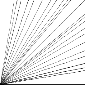
Line segments	Source file
	The $\backslash$ `line` command has two arguments: a direction vector, a length. The components of the direction vector have to be coprime (no common divisor except 1), and they are restricted to the integers $\begin{displaymath} -6,\,-5,\,\dots,\, 5,\,6. \end{displaymath}$ The picture illustrates all 25 possible slope values in the first quadrant. The length is relative to $\backslash$ `unitlength`. The length argument is the vertical coordinate in the case of a vertical line segment, the horizontal coordinate in all other cases. Because of the restrictions to direction vectors, drawing line segments usually necessitates an extensive search for suitable points. In many cases, drawing the desired line segments may not be possible without the use of additional packages, such as `eepic`, or `pstricks`.

Circles	Source file
	The argument of the $\backslash$ `circle` command is relative to $\backslash$ `unitlength` and determines the diameter (not the radius). The original `picture` environment only admits diameters up to approximately 14mm, and even below this limit, not all diameters are possible. The $\backslash$ `circle*` command produces disks (filled circles). As for drawing larger circles, see the section about circles and ellipses.

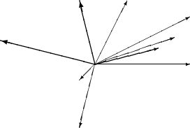
Arrows	Source file
	For arrows, the components of the direction vector are even more restricted than for line segments, namely to the integers $\begin{displaymath} -4,\,-3,\,\dots,\,3,\,4. \end{displaymath}$ Components also have to be coprime (no common divisor except 1). Notice the effect of the `\thicklines` command on the arrows pointing to the upper left.

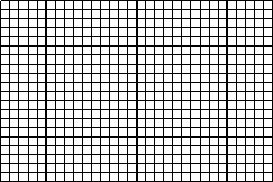
The `multiput` and the `linethickness` command	Source file
	The `\multiput` command has 4 arguments: the starting point, the translation vector, the number of objects, and the object to be drawn. The `\linethickness{`length`}` command applies to horizontal and vertical line segments, but neither to oblique line segments, nor to circles. It does, however, apply to quadratic Bézier curves!

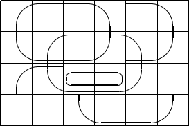
Ovals, `thinlines`, `thicklines`	Source file
	Line thickness can be controlled by two kinds of commands: `\linethickness{`length`}` on the one hand, $\backslash$ `thinlines` and $\backslash$ `thicklines` on the other. While `\linethickness{0.075mm}` applies only to horizontal and vertical lines (and quadratic Bézier curves), `\thinlines` and `\thicklines` apply to oblique line segments as well as to curves such as circles or ovals.

Text, formulas, colors	Source file
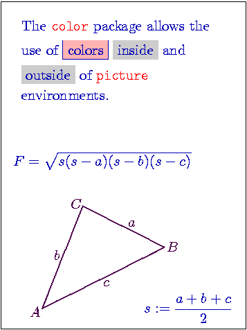
	The `color` package allows the use of colors inside and outside of `picture` environments. Predefined colors of the `color` package are: `black`, `white`, `red`, `green`, `blue`, `yellow`, `cyan`, and `magenta`. As the current example shows, the $\backslash$ `definecolor` command allows for the definition of arbitrary further colors in terms either of the `gray`, or the `rgb` color model. (L^ATEX also supports a third color model, `cymk`). As this example shows, the $\backslash$ `colorbox` and the $\backslash$ `fcolorbox` commands are not compatible with `latex2html`, which produced this text.

Quadratic Bézier curves	Source file
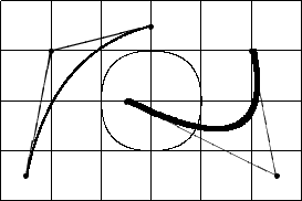
	As this example illustrates, splitting up a circle into four quadratic Bézier curves is not satisfactory. For a better solution, see the section about quadratic Bézier curves. The example again shows the effect of the $\backslash$ `linethickness` command on horizontal or vertical lines, and of the $\backslash$ `thinlines` and $\backslash$ `thicklines` commands on oblique line segments. It also shows that both kinds of commands affect quadratic Bézier curves, each command overriding all previous ones.
Let $P_1=(x_1,\,y_1),\,P_2=(x_2,\,y_2)$ denote the end points, and $m_1,\,m_2$ the respective slopes, of a quadratic Bézier curve. The intermediate control point $S=(x/y)$ is then given by the equations
	(1)
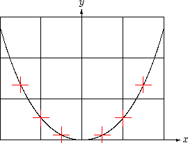
The Java program `qbezier.java` (see PDF Version) started with the line `java qbezier <> <> <> <> <> <>` writes a file `qbezier.tex` which can be pasted into a `picture` environment, whence it draws the desired curve.

Marking angles	Source file
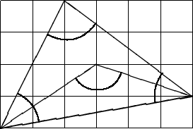
	In the current picture, arcs are approximated by quadratic Bézier curves.
In order to get the control points of an arc of radius $r$ marking the angle $\angle P_1P_2P_3$ , one has to translate and rotate the angle in order to move the vertex to the origin and have the bisector point in the direction of the $x$ axis (transformation $T$ ), reduce the vectors $P_2P_1$ and $P_2P_3$ to length $r$ , let the intermediate control point $P_2$ be equal to $((x_1^2+y_1^2)/x_1, 0)$ , $x_1$ and $y_1$ being the coordinates of point $P_1$ after transformation $T$ and reduction to length $r$ , apply the transformation $T^{-1}$ to points $P_1$ , $P_2$ , and $P_3$ . If the Java program `arc.java` (see PDF Version) is started with the command line `java arc <> <> <> <> <> <> <>`, it produces a file `arc.tex` which can be pasted into a `picture` environment, whence it draws the required arc. As can be seen from the above input file, the obtuse angle is marked in parts: by consequtively marking the angles $\angle(0,\,0)(3,\,2)(3,\,0)$ and $\angle(3,\,0)(3,\,2)(6,\,1)$ .

Line thickness again: the `linethickness` command	Source file
	As can be seen from this picture, the command $\backslash$ `linethickness{`length`}` applies to horizontal and vertical lines as well as to Bézier curves, but not to circles, or oblique line segments. Ovals are a combination of horizontal and vertical lines, and arcs.

Line thickness again: `thinlines` and `thicklines`	Source file
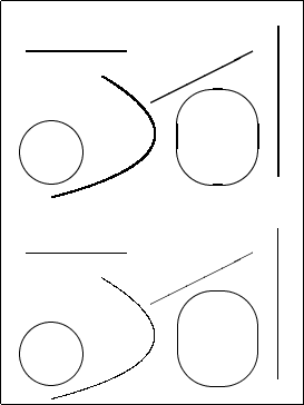
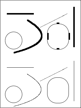
	As the comparison of the lower half of the picture with the upper half shows, the $\backslash$ `thinlines` and the $\backslash$ `thicklines` commands apply to all line segments and curves, but the effect cannot said to be very striking.

Multiple use of predefined partial pictures	Source file
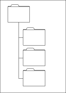
	A partial picture can be declared and defined by the commands `\newsavebox{`name`}` (declaration) `\newsavebox{`name`}(`size`)[`position`]{`content`}` (definition) and then be arbitrarily often used by the command `\usebox{`name`}`. The name argument refers to a L^ATEX storage bin and therefore is of a command nature (which accounts for the backlashes in the current example). size is a numeric pair referring to the current value of `\unitlength`. An object defined with the $\backslash$ `savebox` command (such as `\foldera` in the current example) can be used in the definition of another such element (`\folderb`). The `\oval` command was applied because the connecting segments are two short to be drawn with the `\line` command.

Applications
Falling mass	Source file


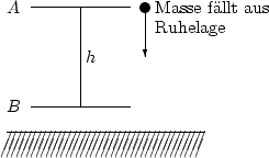
Simultaneousness	Source file


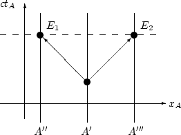
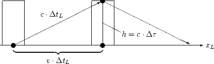
Moving light clock	Source file


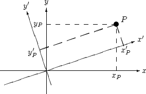
Rotation of axes	Source file


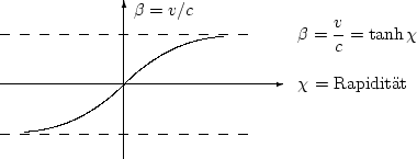
Rapidity	Source file
	Each symmetric half of the `tanh` curve is approximated by a quadratic Bézier curve. See (1) for details.

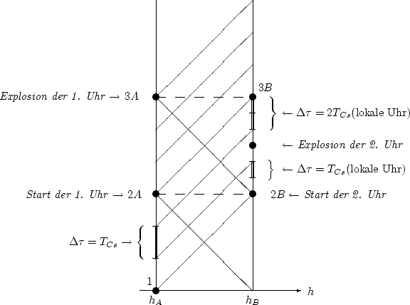
Clocks in gravitational field	Source file


Line of simultaneousness	Source file

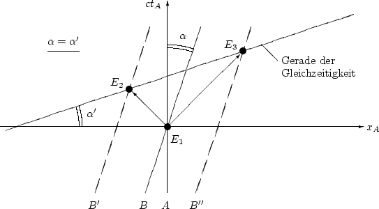
The inserts in the input file drawing the angle markings are produced, according to Marking angles with the Java program `arc.java` (see PDF Version).

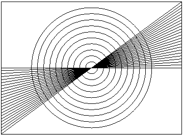
Isotropic spherical waves	Source file


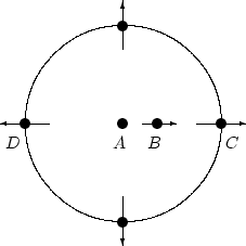
Additional Examples of Bézier Curves
Catenary	Source file
	The right half of the curve ends in the point $(2,\,2.7622)$ , the slope there having the value $m=3.6269$ . Using equation (1) in the section Quadratic Bézier curves, we can calculate the intermediate control points. They turn out to be $(1.2384,\,0)$ and $(-1.2384,\,0)$ . Or, using the Java program `qbezier.java` described there (see PDF Version), we can generate the `qbezier` command lines and insert them into the L^ATEX file. The red crosses indicate points of the real catenary. The error is barely noticeable, being less than one percent.

Forces on the catenary	Source file


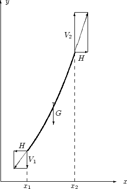
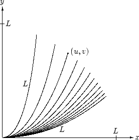
Catenaries of constant length	Source file
	From the equation $\begin{displaymath} \frac{y}{a}=\cosh\frac{x}{a}-1 \end{displaymath}$ of the catenary, it is seen that all catenaries can be obtained by scaling the curve 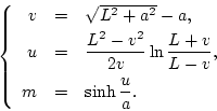$y=\cosh x - 1$ with factor $a$ . A catenary of length $L$ having its vertex in the origin and ending in the point $(u,\,v)$ satisfies (see http://www.vsmp.ch, Bulletin nr. 87) the equations $\begin{displaymath} \left\{ \begin{array}{rcl} v & = & \sqrt{L^2+a^2}-a, \\ [... ... m & = &\displaystyle \sinh\frac{u}{a}. \end{array} \right. \end{displaymath}$
From these equations, for 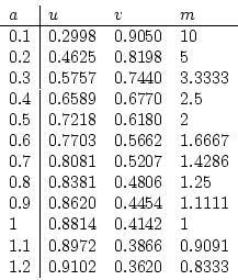$L=1$ we get: $\begin{displaymath} \begin{array}{l\vert lll} a & u & v & m \\ \hline 0.1 ... ...3866 & 0.9091 \\ 1.2 & 0.9102 & 0.3620 & 0.8333 \end{array}\end{displaymath}$ Using equation (1) in the section Quadratic Bézier curves, we can calculate the intermediate control points. Or we can, by using the Java program `qbezier.java` described there (see PDF Version), produce the `qbezier` command lines and insert them into the L^ATEX file.

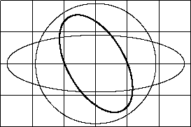
Circles and ellipses	Source file
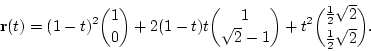
	The circle ( $a=b=1.9$ ) was built from 8 arcs, each of 45 degrees, and each approximated by a quadratic Bézier curve. Circles and ellipses can then be obtained by rotating, scaling and translating.
Thus, the building block of all the circles and ellipses is the quadratic Bézier curve determined by the control points
$\begin{displaymath} \left\{ \begin{array}{rcl} P_1 & = & (1/0),\\ [2mm] P_2 ... ...sqrt{2}\right/\frac{1}{2}\sqrt{2}\right): \end{array} \right. \end{displaymath}$	(2)
45 degrees arc The quadratic Bézier curve with control points (2) is given by the equation $\begin{displaymath} \mathbf{r}(t)=(1-t)^2{1\choose 0}+2(1-t)t{1\choose \sqrt{2}-1} +t^2{\frac{1}{2}\sqrt{2}\choose\frac{1}{2}\sqrt{2}}. \end{displaymath}$ From this, we get:
$\begin{displaymath} \vert\vert\mathbf{r}(t)\vert\vert^2=1+(10-7\sqrt{2})(1-t)^2 t^2, \end{displaymath}$	(3)
$\begin{displaymath} \left\Vert\mathbf{r}\left(\frac{1}{2}\right)\right\Vert^2=\frac{1}{4}\sqrt{26-7\sqrt{2}}\approx 1.003\,135. \end{displaymath}$ The error amounts to approximately 0.3 percent. From (3), we further conclude that $\vert\vert\mathbf{r}(t)\vert\vert>1$ for $0<t<1$ . Letting $t=s+\frac{1}{2}$ , we can see the symmetry with respect to $t=\frac{1}{2}$ : $\begin{displaymath} \vert\vert\mathbf{r}(s)\vert\vert^2=1+(10-7\sqrt{2})\left(s... ...right)^2 \qquad\left(-\frac{1}{2}\le s\le\frac{1}{2}\right). \end{displaymath}$ The Java program `bezierellipsen.java` (see PDF Version) generates a file, `ellipse.tex`, which can be pasted into a `picture` environment. Running the program with `java bezierellipsen <u> <v> <a> <b> <phi>` produces a file representing the ellipse with center $(u/v)$ and radii $a$ und $b$ , and rotated by `<phi>` degrees.

Enhancing the picture Environment with Packages `epic` and `eepic` The packages `epic` and `eepic` enhance the `picture` environment. They are extensively described in GOOSSENS, MITTELBACH, SAMARIN[1]. Two applications of `epic`: `matrixput` and `putfile`
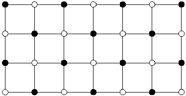
matrixput	Source file
	The `\matrixput` command is the natural generalization of the `\multiput` command to two dimensions. As this example shows, not all the pixels always make it into the final picture.

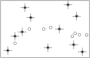
putfile	Source file
The slash in the command `\putfile{data/datafile1}` may have to be replaced by the backslash on a Windows system. The two files `datafile1` and `datafile2` contain one coordinate pair on each line.
	datafile1, for example, contains the lines 10 10 20 20 30 20 35 21 50 15 55 16 52 17 60 16

Line segments and circles in the `eepic` package	Source file
	With the use of the `eepic` package, line segments of any slope (defined by two integers), and circles of any radius can be drawn within the `picture` environment.

Bibliography 1 M. Goossens, F. Mittelbach, A. Samarin The L^ATEX Companion 2 M. Goossens, S. Rahtz, F. Mittelbach The L^ATEX Graphics Companion 3 John D. Hobby, User's Manual, http://cm.bell-labs.com/who/hobby/ 4 Alan Hoenig, TeX Unbound, OXFORD UNIVERSITY PRESS, 1998, ISBN 0-19-509685-1 5 Donald E. Knuth. The METAFONTbook. ADDISON-WESLEY, 1992, ISBN 0-201-13445-4 und ISBN 0-201-13444-6 (soft) 6 Leslie Lampert. L^ATEX - A Document Preparation System. ADDISON-WESLEY, 1994 (13th Printing November 2001), ISBN 0201529831 7 Helmut Kopka. L^ATEX - Eine Einführung. ADDISON-WESLEY, 1992, ISBN 3-89319-434-7 8 Helmut Kopka. L^ATEX - Erweiterungsmöglichkeiten. ADDISON-WESLEY, 1992, ISBN 3-89319-356-1 9 Keith Reckdahl, Using Imported Graphics in LaTeX2e, ftp://ftp.dante.de/tex-archive/info/epslatex.ps, ftp://ftp.dante.de/tex-archive/info/epslatex.pdf

Contents

Basics

Line segments

Circles

Arrows

The `multiput` and
the `linethickness` command

Ovals, `thinlines`, `thicklines`

Text, formulas, colors

Quadratic Bézier curves

Marking angles

Line thickness again:
the `linethickness` command

Line thickness again:
`thinlines` and `thicklines`

Multiple use of
predefined partial pictures

Applications

Falling mass

Simultaneousness

Moving light clock

Rotation of axes

Rapidity

Clocks in gravitational field

Line of simultaneousness

Isotropic spherical waves

Additional Examples of Bézier Curves

Catenary

Forces on the catenary

Catenaries of
constant length

Circles and ellipses

Enhancing the picture Environment with Packages `epic` and `eepic`

Two applications of `epic`: `matrixput` and `putfile`

matrixput

putfile

Line segments and circles
in the `eepic` package

Bibliography